Understanding the Dynamic Balance in Variational Autoencoders

Introduction

Variational Autoencoders (VAEs) are powerful generative models that combine deep learning with probabilistic inference. While their mathematical framework is well-documented, there's a fascinating dynamic that emerges during training: an antagonistic relationship between decoder quality and encoder variance. This blog explores this relationship and its implications for training dynamics.

1. The VAE Framework

At its core, a VAE consists of an encoder that maps inputs to distributions in latent space, and a decoder that reconstructs inputs from sampled latent vectors. The encoder doesn't just compress data - it learns to predict a probability distribution for each input, typically parameterized as a multivariate Gaussian.

2. The Dynamic Balance

The VAE's loss function combines reconstruction quality with latent space regularization:

2.1 Early Training Phase

During early training, when the decoder is still learning, an interesting phenomenon occurs. The system naturally reduces the variance predicted by the encoder to minimize randomness in the latent space. This makes intuitive sense - with a poor decoder, any additional noise in the latent vector makes reconstruction more difficult.

2.2 Later Training Phase

As the decoder improves, it becomes more robust to variations in the latent space. This allows the model to increase the predicted variance without severely impacting reconstruction quality. The improved decoder can handle more diverse latent vectors, enabling better exploration of the latent space.

3. Automatic Curriculum Learning

This dynamic creates an automatic curriculum learning process. The system naturally progresses through different phases:

3.1 Phase 1: Conservative Exploration

Initially, the VAE keeps variance low to ensure stable learning:

3.2 Phase 2: Gradual Expansion

As the decoder improves, the variance gradually increases:

3.3 Phase 3: Equilibrium

Finally, the system reaches a balance between reconstruction accuracy and latent space regularity:

4. Experimental Verification

To verify this dynamic behavior, I've implemented a simple VAE and tracked the evolution of predicted variance during training. The code demonstrates how the variance starts small and gradually increases as the decoder improves.

4.1 Experiment Setup

We implemented a VAE with the following architecture and training configuration:

Model Architecture:

• Encoder: Two-layer MLP (784 → 512 → 256) with batch normalization
• Latent Space: 2-dimensional (for visualization purposes)
• Decoder: Symmetric architecture (2 → 256 → 512 → 784) with batch normalization

Training Parameters:

• Dataset: MNIST (60,000 training samples, 28×28 grayscale images)
• Batch Size: 512
• Optimizer: Adam (lr=1e-3)
• Epochs: 200
• β Values: [0.0, 0.1, 0.5, 1.0, 2.0, 5.0, 10.0]

Loss Function:

The total loss combines reconstruction and KL divergence terms:

where:

• $\mathcal{L}_{\text{recon}} = \text{BCE}(x, \hat{x})$ (Binary Cross Entropy)
• $\mathcal{L}_{\text{KL}} = \frac{1}{2}\sum(1 + \log(\sigma^2) - \mu^2 - \sigma^2)$

4.2 Results Analysis

4.2.1 Training Dynamics

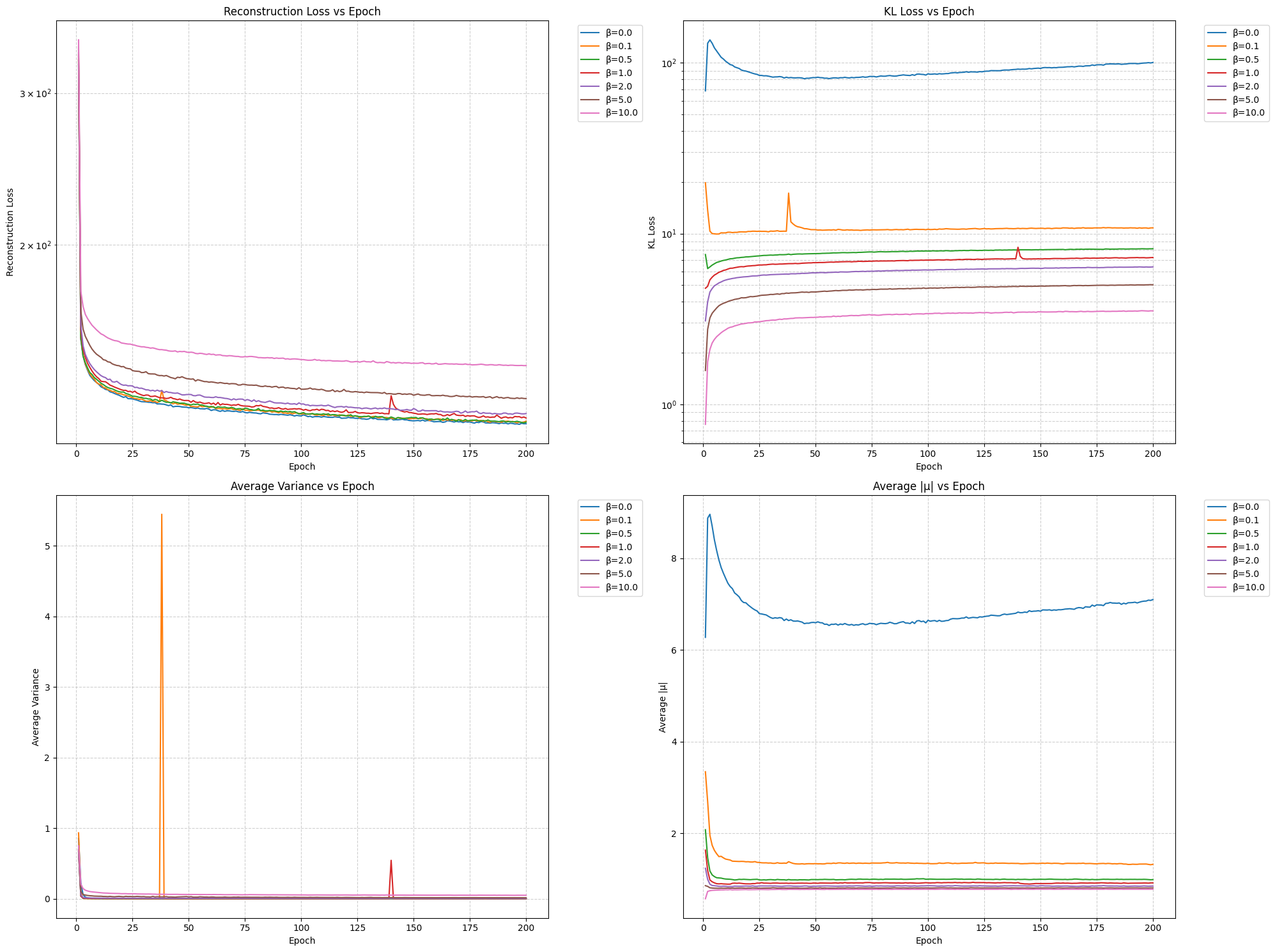
Our first key observation comes from the training loss curves across different β values. Looking at the case where β = 0 (no KL regularization), we observe fascinating dynamics:

Figure 1: Training curves showing reconstruction loss (left) and KL divergence (right) for different β values. Note how the KL divergence reaches around 100 when β = 0, and the unique variance behavior without regularization.

These results empirically validate our theoretical analysis from Section 2. Without KL regularization:

• The encoder's predicted variance initially decreases, then notably increases in later training stages
• The KL divergence term grows to approximately 100, far from the desired unit Gaussian behavior
• This behavior suggests the encoder is actively increasing variance to push the decoder toward learning more robust features

4.2.2 Impact of KL Regularization

When we introduce KL regularization (β > 0), we observe a clear stabilizing effect on the variance. But does this regularization actually improve the model's performance? The generated samples provide compelling evidence:

Figure 2a: Generated samples with β = 0. Note the blurrier, less defined digit structures.

Figure 2b: Generated samples with β = 1. Observe the sharper, more well-defined digits.

4.2.3 Latent Space Organization

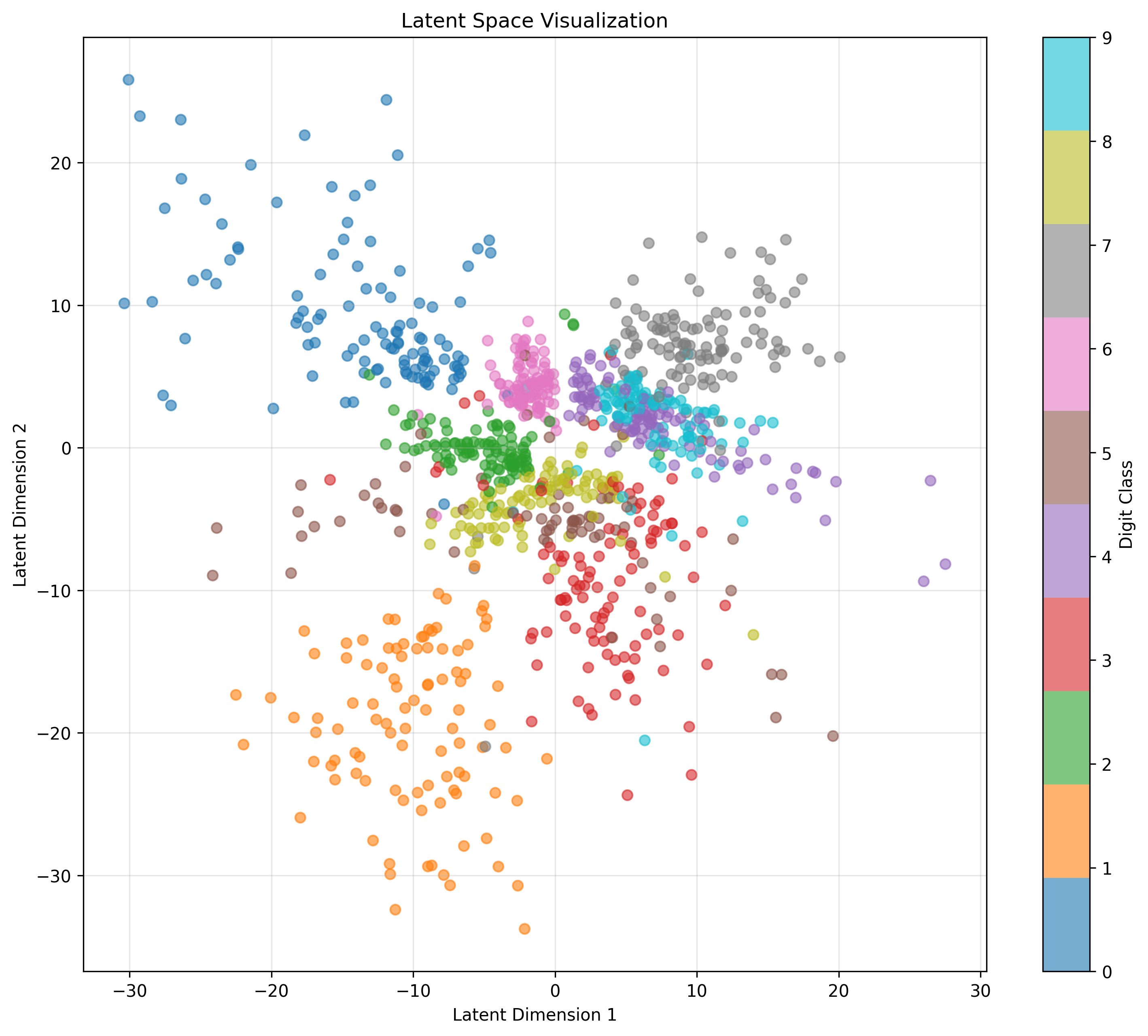
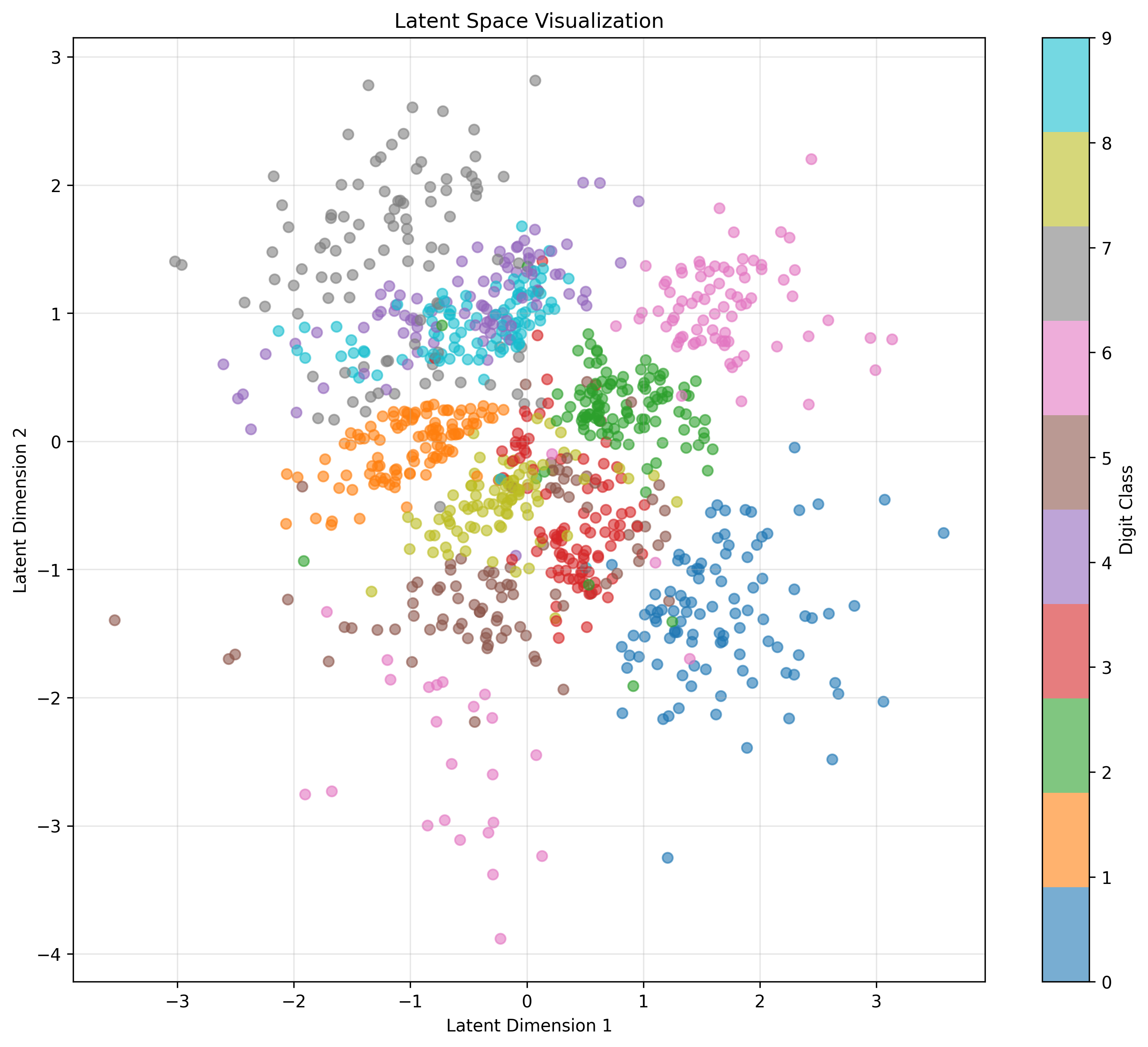
The latent space distributions provide further insight into the effect of KL regularization:

Figure 3a: Latent space distribution with β = 0, showing irregular clustering and spread.

Figure 3b: Latent space distribution with β = 1, exhibiting Gaussian-like structure.

The latent space visualizations reveal that with β = 1, the distribution much more closely approximates our desired unit Gaussian prior. This structured organization of the latent space contributes to the improved quality of generated samples, as the decoder learns to map from a more regular distribution.

5. Practical Implications

Understanding this dynamic balance has several important implications for VAE training:

• Training Stability: The automatic variance adjustment helps maintain stable training by matching the latent space complexity to decoder capability.
• Quality Assessment: The evolution of predicted variance serves as a useful metric for monitoring training progress.
• Architecture Design: Decoder capacity should be matched to the desired latent space complexity, as it ultimately limits the sustainable variance.

Conclusion

The antagonistic relationship between decoder quality and encoder variance in VAEs creates an elegant self-regulating system. This automatic curriculum helps the model progress from simple to complex representations, contributing to the stability and effectiveness of VAE training. Understanding this dynamic can help in better architecture design and training process monitoring.

This phenomenon also raises interesting questions about similar dynamics in other generative models. Do other variational methods exhibit similar self-regulating behavior? How can we leverage this understanding to design better training procedures? These questions point to exciting directions for future research.

  @misc{vae-dynamics-demo,
    author    = {Tianrun Hu},
    title     = {Understanding the Dynamic Balance in Variational Autoencoders},
    year      = {2025},
    publisher = {GitHub},
    url       = {https://h-tr.github.io/blog/posts/vae-dynamics.html}